Convolution from Scratch: Math, Images, and Kernels
1. Introduction
Convolution is a mathematical operation that takes two inputs and produces a third. One input is the signal, the data we want to transform. The other is the kernel (also called a filter) a small set of weights that defines how the signal is transformed. The output is a new signal where, at every position, the kernel has been applied to the local neighbourhood of the original signal.
More concretely: the kernel slides across the signal step by step. At each position, it computes the dot product between itself and the local part of the signal it currently overlaps. That single number becomes the output at that position.
What makes this powerful is what the kernel encodes. A kernel that averages its neighbourhood blurs the signal. A kernel that computes differences between adjacent values detects edges.
This blog focuses on building the full picture from scratch on how convolution works in computer vision and how it helps to extract different features from images.
2. The Mathematics of Convolution
2.1 Continuous Convolution
For two continuous functions f and g, convolution is defined as:
$$(f * g)(t) = \int_{-\infty}^{\infty} f(x) \cdot g(t - x) , dx$$
At every output point t, we compute a weighted integral of f, where the weights come from g, flipped and shifted to position t. The flip (substituting t - x instead of x) is what makes it convolution rather than cross-correlation. In image processing, this distinction is often ignored because most kernels used in practice are symmetric.
2.2 Discrete Convolution
In practice, signals and images are discrete, finite grids of numbers. The discrete form is:
$$(a * b)n = \sum{\substack{i, j \ i + j = n}} a_i \cdot b_j$$
Every output value at index n is a sum over all pairs (i, j) from the two sequences that add up to n. This is the form that maps directly to how images are processed.
2.3 Signal and Kernel
In computer vision, one input is the signal, the data being processed (an image ) and the other is the kernel ( a compact description of the transformation being applied ). The kernel is almost always much smaller than the signal.
The key insight: convolution is a local operation. Each output value depends only on a small neighbourhood of the input, not the entire signal. This locality is precisely what makes it so useful in image processing to extract features. In traditional CV an image is said to have localised features (edges, corners, textures) that can be detected by applying the right kernel to the right neighbourhood.
3. Images as Matrices
Before applying convolution to images, let us understand how images are represented numerically.
3.1 Grayscale Images
A grayscale image is a 2D matrix of shape Height * Width, where each element is a pixel intensity value in the range [0, 255] , 0 is black, 255 is white, and everything in between is a shade of grey.
[  0,   0,   0,   0,   0 ]
[  0,  50, 120, 200,   0 ]
[  0,  80, 255, 180,   0 ]
[  0,  40, 100,  60,   0 ]
[  0,   0,   0,   0,   0 ]
Each row is a horizontal strip of pixels. Each column is a vertical strip. The value at position (i, j) is the brightness of the pixel at row i, column j.
3.2 RGB (Colour) Images
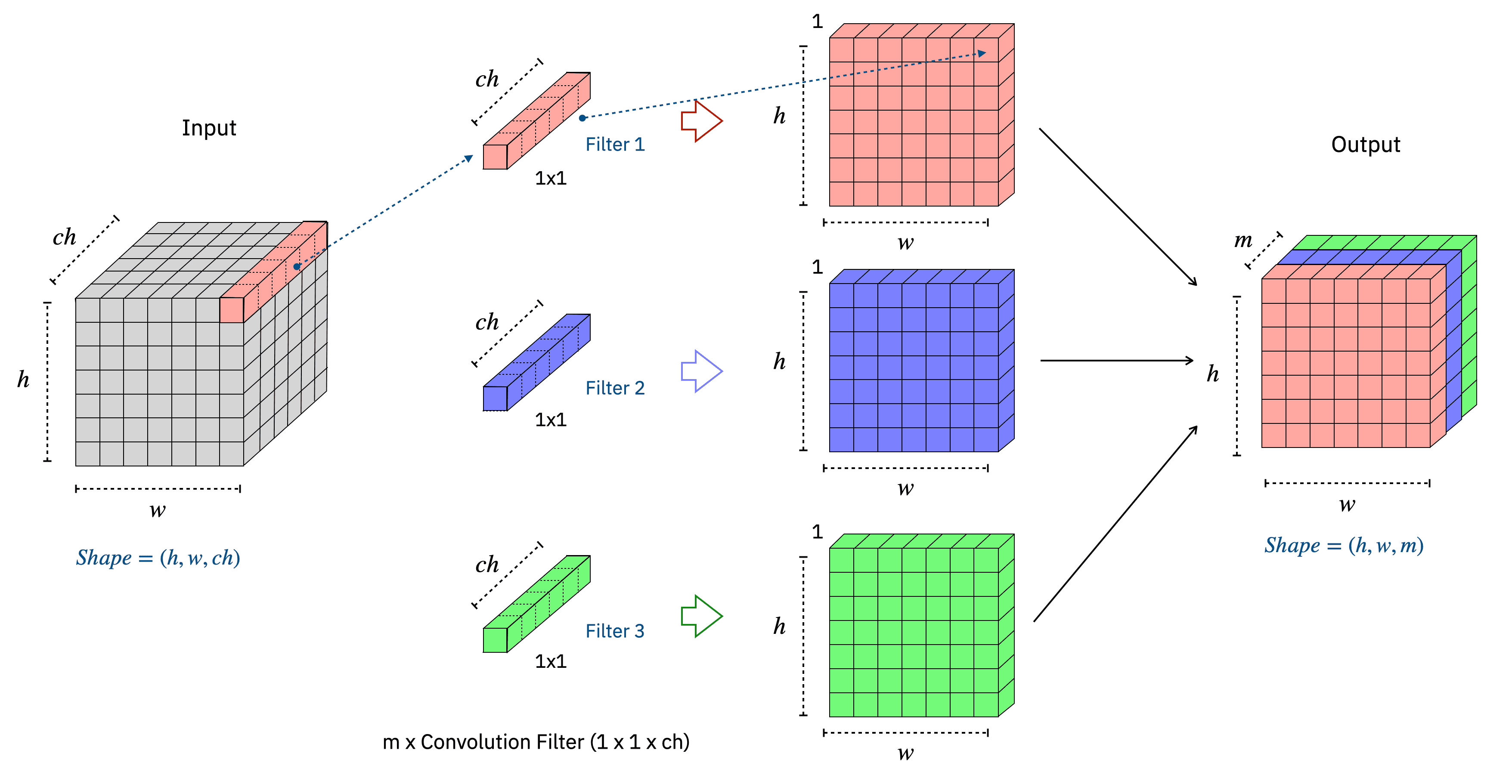
A colour image adds a third dimension, the channel. An RGB image has shape Height*Width*3-channels, where the three channels represent Red, Green, and Blue intensities respectively.
$$\text{Image} \in \mathbb{R}^{H \times W \times C}$$
where C = 3 for RGB and C = 1 for grayscale.
Each channel is its own Height *Width matrix. When a convolution kernel is applied to a colour image, it operates independently on each channel.
4. Convolution in Computer Vision
4.1 The Sliding Window
Given an input image of size N*N and a kernel of size K*K, we slide the kernel across every valid position. At each position (i, j), the output value is:
$$\text{Output}(i,, j) = \sum_{m=0}^{K-1} \sum_{n=0}^{K-1} \text{Input}(i + m, j + n) \cdot \text{Kernel}(m, n)$$
The kernel acts as a template of weights. High positive weights amplify matching patterns. Negative weights suppress or invert them. Zero weights ignore those positions entirely. The specific pattern a kernel responds to depends entirely on what values are in it.
4.2 Stride
Stride S controls how many pixels the kernel moves at each step. With S = 1, the kernel moves one pixel at a time.
4.3 Output Size
With input size N, kernel size K, padding P, and stride S, the output dimension is:
$$\text{Output size} = \left\lfloor \frac{N + 2P - K}{S} \right\rfloor + 1$$
Without padding (P = 0) and with stride 1, this simplifies to:
$$\text{Output size} = N - K + 1$$
A 5 5 image convolved with a 3*3 kernel gives a 3*3 output. Stack ten such layers and the spatial dimensions collapse to a point. This is the shrinking problem and why padding exists. We will address it in detail in Section 6, after we understand what kernels actually do.
4.4 Why Odd Kernels Only
For the output to have the same spatial size as the input (with stride 1), we need:
$$P = \frac{K - 1}{2}$$
This requires K to be odd to yield an integer. Even-sized kernels have no clean centre pixel, create asymmetric padding, and are harder to reason about geometrically. In practice, always use odd kernels: 3*3, 5*5, 7*7.
How Convolution Operation works
https://codepen.io/AK-Notion/pen/WbovLQm
5. Kernels
"A kernel is a local weighting rule is, output pixel = sum (local pixels*weights)"
The values inside a kernel encode a specific transformation. The weights determine what the convolution amplifies, suppresses, or detects.
Before we look at specific kernels, here is the image we will use throughout this section to make the effects concrete
Original image used for examples
Every kernel output shown below is produced by applying that kernel to this same image, so the effects are directly comparable.
5.1 The Weights Encode Intent
Before examining individual kernels, it helps to understand what the weight matrix geometry means:
A positive center, negative surroundings → the kernel responds to pixels that differ from their neighborhood (edge / sharpening behavior)
All positive, summing to 1 → the kernel averages its neighborhood (blur behavior)
Positive on one side, negative on the other → the kernel responds to directional intensity changes (gradient / edge detection in one direction)
Asymmetric weights → the kernel has a directional bias
i. Box Blur
$$K_{\text{box}} = \frac{1}{9}\begin{bmatrix} [1,1,1] , [1,1,1], [1,1,1] \end{bmatrix}$$
Every weight is equal: 1/9. The output at every pixel is the uniform average of it and its 8 neighbors. No position is weighted more than another.
What it does: Replaces each pixel with the mean of its local neighborhood. This removes high-frequency detail (noise, sharp edges) because rapid local variations get averaged out.
Limitation: Treats all neighbors as equally important regardless of distance. A pixel two positions away influences the output just as much as the immediately adjacent one. This produces a blocky, artificial-looking blur.
Box blur (3×3 uniform average)
ii. Gaussian Blur
$$K_{\text{gaussian}} = \frac{1}{16}\begin{bmatrix} [1,2,1], [2,4,2], [1,2,1] \end{bmatrix}$$
The weights follow a 2D Gaussian (bell curve) distribution, highest at the center, falling off with distance. The center pixel contributes weight 4, immediate neighbors weight 2, and corners weight 1.
What it does: A spatially weighted average where proximity matters. The result is a smoother, more natural-looking blur than the box kernel.
Why it matches the physical world: Gaussian blur models natural diffusion processes like optical defocus, heat diffusion, sensor noise. Real-world blur is rarely uniform; closer pixels in a neighborhood really do belong together more than distant ones. It reduces local variance (noise) without destroying structural information as aggressively as box blur.
A deeper note on blur kernels in general: All blur kernels share a common assumption, that neighboring pixels are likely to have similar values (they belong to the same surface, material, or object). By pulling each pixel toward its neighbourhood average, blur kernels reduce local variance. This is a form of signal smoothing, and it is why blurring before edge detection makes the subsequent edge detector more robust.
Gaussian blur (spatially weighted average)
iii Sobel X and Sobel Y — Edge Detection via Gradients
The Sobel kernels detect edges by approximating the first-order derivative (gradient) of image intensity. A large gradient at a pixel means intensity is changing rapidly which is the definition of an edge.
Sobel X — detects vertical edges by measuring how intensity changes left to right:
$$K_{Sx} = \begin{bmatrix} [1 ,0,-1], [2,0,-2], [1,0,-1] \end{bmatrix}$$
Sobel Y — detects horizontal edges by measuring how intensity changes top to bottom:
$$K_{Sy} = \begin{bmatrix} [1,2,1], [0 ,0 , 0],[-1, -2 ,-1] \end{bmatrix}$$
Reading the kernel structure:
The left column of SobelX matrix is [+1, +2, +1] and the right column is [-1, -2, -1]. The centre column is zero. The kernel is literally computing the difference between the left side and the right side of the patch.
The +2 and -2 in the center of the row give more weight to the pixel directly adjacent (horizontally), reducing noise sensitivity compared to the corners.
Sobel Y is the transpose of Sobel X the same logic, rotated 90°.
Output: Where intensity is uniform, the dot product is close to zero (dark in the output). Where there is a sharp left-right boundary, it is large (bright in the output). The result is a gradient map: bright regions are edges, dark regions are flat.
Sobel X rocks image
Sobel Y rocks image
iv. Laplacian Kernel — Edge Detection via Second Derivative
$$K_{\text{Laplacian}} = \begin{bmatrix} [0 ,1, 0], [1 ,-4, 1] , [0,1, 0] \end{bmatrix}$$
Where Sobel detects where intensity changes, the Laplacian detects where the rate of change changes the second derivative.
Reading the kernel: The center weight is \(-4\) and the four cardinal neighbors are +1. The kernel computes:
$$(f_\text{left} + f_\text{right} - 2f_\text{centre}) + (f_\text{top} + f_\text{bottom} - 2f_\text{centre})$$
This is the discrete approximation:
$$\nabla^2 I = \frac{\partial^2 I}{\partial x^2} + \frac{\partial^2 I}{\partial y^2}$$
What it detects: Regions where intensity is rapidly accelerating or decelerating the peaks and troughs of the gradient. It fires at both sides of an edge (the transition in and the transition out), making it sensitive to fine detail and texture in all directions simultaneously unlike Sobel which is directional.
Tradeoff: The second derivative amplifies noise more aggressively than the first. In practice we always apply a Gaussian blur before the Laplacian. This combination has a name: Laplacian of Gaussian (LoG).
Laplacian edge detection
6. Padding
We saw in Section 4 that convolving an N*N image with a K*K kernel (no padding, stride 1) produces an (N - K + 1) * (N - K + 1) output. Every layer shrinks the image. In a deep network, this is a problem as the spatial information is progressively destroyed before the network has had a chance to extract it.
Padding solves this by adding extra pixels around the border of the image before convolution, so the output can be made to match the input size.
To pad by P pixels:
Add P rows on top and P rows on bottom
Add P columns on the left and P columns on the right
A 5*5 image with P = 1, becomes 7*7 before convolution. Applying a 3*3 kernel then gives a 5*5 output
The question now would be: what values do we use for those extra pixels? Different strategies make different assumptions about what the padding pixels beyond the original image boundary.
i. Zero Padding (Dirichlet Boundary Condition)
The simplest approach: pad with zeros. Pixels outside the image are treated as black.
$$\tilde{x}(i, j) = \begin{cases} x(i, j) & \text{if } 0 \leq i < H,\ 0 \leq j < W \ || 0 & \text{otherwise} \end{cases}$$
Scientific name: Dirichlet boundary condition.
ii. Replication Padding (Neumann Boundary Condition)
Border pixel values are extended outward the edge of the image is replicated into the padding region.
$$\tilde{x}(i, j) = x\big(\text{clamp}(i,\ 0,\ H-1),\ \text{clamp}(j,\ 0,\ W-1)\big)$$
where the clamp function restricts any index to the valid range:
$$\text{clamp}(a, l, r) = \min(\max(a, l), r)$$
If an index is negative, it snaps to 0. If it exceeds H-1 or W-1, it snaps to the last valid index. The result: the border pixel is copied into all padding positions along its row or column.
Intuition: Assumes the world beyond the image boundary is a flat continuation of the edge. Avoids the dark border artifact of zero padding.
Scientific name: Neumann boundary condition.
7. End-to-End Code Example
Below is my NumPy implementation of 2D convolution, no deep learning libraries.
import numpy as np
import cv2

imgPath = "rocks.jpg"

def calculate_padding_length(n: int) -> int:
    if n == 0 or n%2 == 0:
        return -1
    return (n-1) // 2

def build_new_image_matrix_with_reflect_padding(img: np.ndarray, pad: int) -> np.ndarray:

    padded_matrix = np.pad(img, ((pad, pad), (pad, pad), (0,0)), mode='reflect')
    return padded_matrix

def BoxBlurConvolute(img: np.ndarray) -> np.ndarray:
    """Given a n*n matrix return a clipped output matrix, which is a result of convolution operation"""
    kernel = np.array([
        [1/9, 1/9, 1/9],
        [1/9, 1/9, 1/9],
        [1/9, 1/9, 1/9]
    ], dtype=np.float32)

    k = kernel.shape[0]
    h,w,c = img.shape

    padding_length = calculate_padding_length(len(kernel))
    if padding_length <= 0:
        raise "Error with padding length"

    paddedImg = build_new_image_matrix_with_reflect_padding(img, padding_length)

    output = np.zeros(img.shape, dtype=np.float32)

    for i in range(h):
        for j in range(w):
            region = paddedImg[i:i+k,j:j+k]
            for ch in range(c):
                output[i,j,ch] = np.sum(region[:,:,ch] * kernel)

    output = np.clip(output,0,255).astype(np.uint8)

    return output

def GuassianBlurConvolute(img: np.array) -> np.ndarray:
    """ Gaussian Blur, where the emphasis is on nearby pixels than the distant ones"""
    kernel = np.array([
        [1/16,2/16,1/16],
        [2/16,4/16,2/16],
        [1/16,2/16,1/16],
    ],dtype=np.float32)

    k = kernel.shape[0]
    h,w,c = img.shape

    paddingLength = calculate_padding_length(k)
    if paddingLength < 0:
        raise "Error calculating padding length"

    paddedImg = build_new_image_matrix_with_reflect_padding(img,paddingLength)

    output = np.zeros(img.shape, dtype=np.float32)

    for i in range(h):
        for j in range(w):
            region = paddedImg[i:i+k,j:j+k]
            for ch in range(c):
                output[i,j,ch] = np.sum(region[:,:,ch] * kernel)

    output = np.clip(output,0,255).astype(np.uint8)

    return output

def SobelXConvolute(img: np.array) -> np.ndarray:
    """ It highlights vertical edges. """

    kernel = np.array([
        [1,0,-1],
        [2,0,-2],
        [1,0,-1],
    ], dtype=np.float32)

    k = kernel.shape[0]
    h,w,c = img.shape

    paddingLength = calculate_padding_length(k)
    paddedImg = build_new_image_matrix_with_reflect_padding(img,paddingLength)

    output = np.zeros(img.shape,dtype=np.float32)

    for i in range(h):
        for j in range(w):
            region = paddedImg[i:i+k,j:j+k]
            for ch in range(c):
                output[i,j,ch] = np.sum(region[:,:,ch] * kernel)

    output = np.clip(output,0,255).astype(np.uint8)

    return output

def SobelYConvolute(img: np.array) -> np.ndarray:
    """ It highlights horizontal edges. """

    kernel = np.array([
        [1,2,1],
        [0,0,0],
        [-1,-2,-1],
    ], dtype=np.float32)

    k = kernel.shape[0]
    h,w,c = img.shape

    paddingLength = calculate_padding_length(k)
    paddedImg = build_new_image_matrix_with_reflect_padding(img,paddingLength)

    output = np.zeros(img.shape,dtype=np.float32)

    for i in range(h):
        for j in range(w):
            region = paddedImg[i:i+k,j:j+k]
            for ch in range(c):
                output[i,j,ch] = np.sum(region[:,:,ch] * kernel)

    output = np.clip(output,0,255).astype(np.uint8)

    return output

def LaplaceConvolute(img: np.array) -> np.ndarray:
    """ Detect regions where intensity changes rapidly """

    kernel = np.array([
        [0,1,0],
        [1,-4,1],
        [0,1,0],
    ], dtype=np.float32)

    k = kernel.shape[0]
    h,w,c = img.shape

    paddingLength = calculate_padding_length(k)
    paddedImg = build_new_image_matrix_with_reflect_padding(img,paddingLength)

    output = np.zeros(img.shape,dtype=np.float32)

    for i in range(h):
        for j in range(w):
            region = paddedImg[i:i+k,j:j+k]
            for ch in range(c):
                output[i,j,ch] = np.sum(region[:,:,ch] * kernel)

    output = np.clip(output,0,255).astype(np.uint8)

    return output

def main():
    img = cv2.imread(imgPath)
    img = img.astype(np.float32)
    boxBlur = BoxBlurConvolute(img)
    gaussianBlur = GuassianBlurConvolute(img)
    xAxisEdge = SobelXConvolute(img)
    yAxisEdge = SobelYConvolute(img)
    laplaceConvolution = LaplaceConvolute(img)


    cv2.imshow("Original Image", img.astype(np.uint8))
    cv2.imshow("Convolution Image", boxBlur)
    cv2.imshow("Gaussian Blur Image", gaussianBlur)
    cv2.imshow("Sobel X Convolution", xAxisEdge)
    cv2.imshow("Sobel Y Convolution", yAxisEdge)
    cv2.imshow("Laplace Convolution", laplaceConvolution)
    cv2.waitKey(0)
    cv2.destroyAllWindows()

if __name__ == "__main__":
    main()
8. Conclusion
Convolution is a deceptively simple operation, slide a kernel, compute a dot product. It underpins almost everything in computer vision